The extraordinary brightness of Venus as the evening star invoke many assorted fantasies. Lovers dreams about a paradise on the Venus, which is an island in the universe darkness. For peoples believing on Martians, Venus setting appears as a landing of its spacecraft. Venus looks as in fast motion, especially, when Venus is observed in some clouds. Venus setting can be also very impressive for painters, photographers and astronomers. The magic performance of ambient light, twilight sky, surroundings and Venus itself offers the absolutely extraordinary experience.
I spend one evening with Venus by observing of the setting and many days and evenings with processing (and related business) of acquired images. My primary goal of the observation was pointed on visual demonstration of an astronomical refraction. The follow-up processing has been inspired me to mining more information from collected images.
SnapshootingTo acquire of nice sequence of refracted Venus, I selected
Kotvrdovice's airport what
I visited some time ago. The place offers relative good altitude about 560 meters over sea level, so I expected perfect horizon together with a separated place available by a car. Kojál top at proximity has the no separation, place to parking and is close to a road. The expecting Venus setting point is situated in direction of south part of
Moravian Karst with low air (light) pollution.
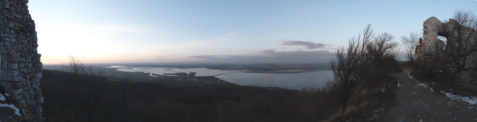
View Larger MapI pitch my tripod at point 16:47:20.1 E, 49:21:52.1 N. The place is on a rural road and on a local ridge near of a hunter's hide. The first snapped image shows a scenery at moment after my arrival.
 The first image.
I manually grabbed a set of images for every minute with start about 15:35 UT and finish at 17:18 UT (but see next note!). Total 101 images has been acquired. Canon EOS 30D has been used with lens EF-S 18-55mm, f/5.7 without any zoom, ISO 1600, a minimal diaphragm. Exposures times has been changed during a light fade of the twilight as I completed into the table:
15:35-15:49 15 1/100
15:50-16:00 9 1/10
16:01-16:15 13 1/2
16:16-16:39 23 4
16:40-17:18 38 8
 An air view to Kotvrdovice's airport. The hide is on left part between the airport's facility and a wood. Kojál transmitter at left top corner, a village Krásensko at top, a small part of Senetářov and Kotvrdovice on right edge from top to bottom (in this order).
Unfortunately, I forget done any time synchronisation of a interval clock of the camera before or after of the trip. So precise time synchronisation is lost forever. Fortunately, I check of time on my mobile phone at start of observation but for information purposes only, without required (on second) precision. It means that all times are considered to be inaccurate (± 30sec). The relative precision is better than 1 sec.
PreprocessingI acquired all images manually by clicking of button on Canon's body. So I expected that the images can be each other shifted. Therefore, I used the translation property of a cross correlation of
Fourier transformation of images to precise co-add of all images to same origin. So, I created of the forward FFT of reference and working copy images. The
Hanning window function has been used for bottom part of original images. The phase-correlation and backward FFT followed. Finally, shifts has been computed as centroids of delta function-like peak.
Shifts has been released only for integer segments. I expecting that precision would be not grow, if a non-integer shifts will be used and interpolation would be degrade sharp features of the output image.
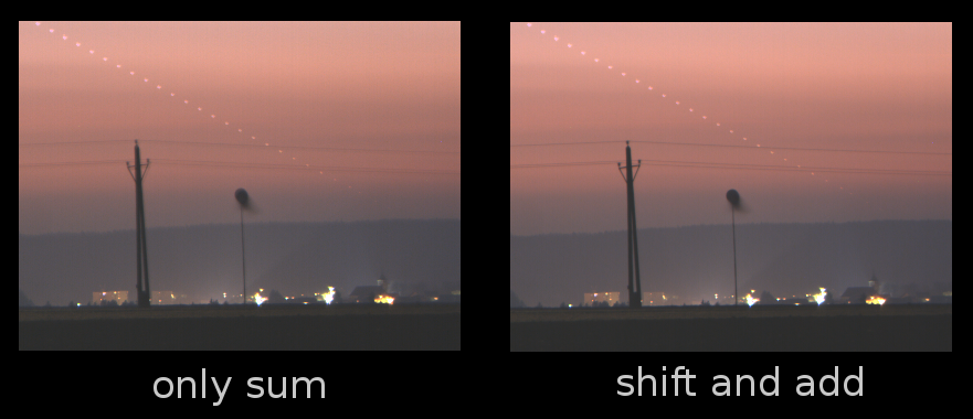
An example of sum of images with and without shifts is shown on the zoomed subimage. The image on the left is simple co-add of all images while the right image shows shifted and co-added images. In my opinion, the careful preprocessing leaded to a little bit sharper picture.
The displacement of color layers worked well when I used all colors together of weighted by white multiplication factors (eg. on grayscale images). Initially, I tried to get shifts for every color layer individually and than compute the mean between its. I expected a fine shift due to Bayer mask, but the shift showed some random behavior as a perhaps product of a noise.
The final image has been created by a method analogous to Iris function
ADD_MAX by Ch. Buil. Simply, the output image is not only sum (or mean) of two images but one gets the brighter pixel of images. The method grows intensity of a potentially moving inter-image object (Venus). Without this, the Venus trace will be lose on evening sky. However, final colors of the (variable) sky background may be very strange.
The white balance parameters provided by the camera gives not satisfactory color balance. Therefore I equalized the image by hand. Usually on a white object on images like Venus or by automatic way with -fr parameter of fitspng.
The most important part of the processing is on base of my specific routines. I'm attaching
link for an inspiration.
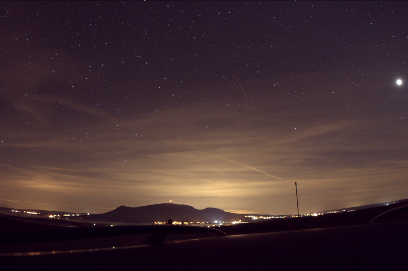
 Venus setting on 15 Nov. 2008 . This composed image shows track of Venus (central body) above south-west horizon at Kotvrdovice's (CZ) airport. The chain of pearls has origin in short exposures of Venus in one-minute intervals. We can see that the finish of observed path is raised with respect to expected (by following of beginning part) one. It is exhibition of the astronomical refraction of the light in Earth's atmosphere. The track also shows decreasing of amount of the light and its reddening during the setting. Both effects are product of scattering and absorption of light in air. Read the post for detailed description.
The astrometric calibration has been done by Gaia software on grayscale version of one of latest images including some stars. The calibration shows that a projection of the lens is gnomonical with precision better than 2-3 arcmin/pixels. A scale is 0.0165 deg/pix = 0.99 '/pix (minute per pixel). A field of view is 29°×19°. The center of the calibrated image is at coordinates 19:13, -26:00 at 17:17 UT (time epoch). Equatorial coordinates has been rotated about 25° to image's coordinates. The image itself is rotated around vertical (horizontal coordinates) by approximate 1°. The parameters are visualised on the image:
 Astronomical refraction
The main goal of my work is to show effect of the astronomical refraction. It can be easy obtained by observing of any point source in time, but when the object downwards really slowly with acute angle to horizon, the observed path may be visibly deviated from non-refracted one. The deflection is nicely demonstrated on annotated images:


Technically, the refraction can be described on a graph of dependence between the observed and the true (not affected by the refraction) zenith distance of some object. The expected values has been computed by a standard way from linearly interpolated coordinates of Venus by NASA's
Horizonts. It agrees with values by Xephem.
Measured coordinates has been derived from grayscaled images. I estimated centroids of Venus by the weighted mean. The error of the determination is order of tenth of pixels/arcmin.
The next step is computation of the zenith distance (or elevation) of Venus. In principle we can use two methods:
- Plain. Using by a scale and a simple geometry, we determine distances in pixels of Venus and horizon. The Euclidean geometry with only rotations and translations is used.
- Gnomonic. Using by known rectangular coordinates and the gnomonic transformation, we determine equatorial coordinates together with transformed to horizontal coordinates.
Both methods may include some systematic errors. Simple plain geometry has known deviations from spherical coordinates when angles gets values over five degrees. The gnomonic transformation fits spherical coordinates by the better way, but we are not sure that our object lens display some scene by the expected way.
The results of both methods of determination zenith distance from photographic plate are plotted in refraction graph. The plain method shows nonlinear great residua and it is clearly unusable. The gnomonic method is little bit better but there are still great differences.

I also plot of Bennett's approximation of the refraction formula according to Astronomical Algorithms by J. Meeus. Other simple refraction laws on base of tangents of the zenith distance (one or tree order) are unusable in the range of observed quantities.
The visible discrepancy between the approximation and observation has unclear origin. The statistical errors are visualised by random noise. I notices relative higher noise on beginning of observation how it vanished when the ratio of signal to noise is growing. I expected that the refraction will affected by some clouds near of the horizon. Nevertheless, the appropriate part of the measured curve is nicely smooth.
The discrepancy is not due to uncertainly on time determination (the change a few minutes minute slightly modified profile but not importantly). It is also valid for changes in an atmospheric pressure and an ambient temperature.
Only for information, I tried to fit the data by any way. A final fit is a set of points tightly reproducing of the Bennett's approximation. The fit has two free parameters: The relative time between the astrometry approximation and observation times has been changed relative about minute (this is principally incorrectly). The change leaded to a little bit deflection of refractive curve so the profile is more similar to the Bennett's approximation. As second free parameter, a vertical shift of 7 pixels/arcmin has been used (also it is uncorrected again).
My own hypothesis of explaining of the measurements is a non-precise model of the (gnomonical) projection. Firstly, I assumed that the projection is gnomonical on full area of the chip. The assumption may be wrong. The gnomonic projection strongly deforms area elements far from center of projection. Therefore, manufacturers can use any different kind of the projection. For example, some "mean" between the gnomonic and a stereographic projection may be used. Secondly, the fitting routine of Gaia assumed such model of the gnomonical projection which have different scales in Right Ascension and Declination, but my images are deformed in some another direction. The images are squeezed in the vertical direction by the refraction. It leads us to use of a model which will be correctly describe the refraction during of gnomonic projection determination. Simply, we can say that the vertical scale will not be more linear, but it will varied with the zenith distance. The construction of the model will not complicated but I abandoned its due to some uncertainty in the time determination and due to low number of stars near of horizon, so I assume, that the corrected method will not give significantly better results.
The refraction itself is a very fascinating field of applied optics. I recommends visit of
wikipedia page and
pages of Andrew T. Young about refraction.
PhotometryWhen the light of a setting object pass trough layers of atmosphere, the observer can detect an exponential attenuation of light together with a color change of the object. Both effect are clearly visible on composed image above.
I think than more better visualisation is represented by a standard photometric analysis of images. By the way, I done an aperture photometry by obvious method (simpler version of one implemented in Munipack). The output magnitudes has been normalized by exposure time and calibrated by the known extratmospheric visual magnitude (again by Horizont) of Venus in G band. I didn't used color balance factors and subtract of a dark frame because the ambient temperature varied about ten degrees. I only subtracted a bias of images which I assumed on level 128 for a RAW image.
The spectral sensitivity of Canon EOS 30D is not available. Therefore, I assumed that the property is similar to one of
EOS 300D. I approximated the sensitivity in R band by Gaussian with its center on 600 nm and its half-width about 30 nm, G band as then rectangle with the height 100% and in the range 500 - 600 nm and B band as the rectangle with the height 75% and the width 430 - 480nm. By the way, I get correction color indexes as 0.27, 0, -0.38 for R, G, and B magnitudes and a black body on the temperature of Sun. The reliability is low, so the color indexes may contains systematic deviations of order of tenth magnitude.

The instrumental magnitudes has been calibrated via extinction lines in range of 9 to 30 airmasses. To estimate of the airmass I used formula by (perhaps)
Young(1994) , see also article on
wikipedia. The least square fitting gives following values extinction coefficients in all bands:
B 0.188± 0.003
G 0.114 ± 0.004
R 0.090 ± 0.003
The first part of graph doesn't follow the extinction law and the magnitudes are perhaps absurd. I think that this is the demonstration of effect described in my
previous post. It is simply due to extremal height level of background with comparison to the light signal of Venus.
Sky's brightnessThe last graph shows surface magnitude of sky near of top of my images (at elevation ten degrees). I selected a rectangular angular area with constant position. The selected magnitudes shows expected profile. The uncertainty may by a few of tenth of magnitude. The values in minimum are a few magnitudes over natural sky. It may be due to really dark sky when the camera detect thermal noise only or the sky may be illuminated by a near village or a town. Note that when Venus set, the Moon has raised on opposite point of the sky.
 Color index
The last graph shows dependence of color indexes on time. I note that the numbers has different base than classical astronomical color bands. Only relative changes can by surly determined from the profiles.
The profiles of Venus shows strong evidence for reddening as we expected from visual determination. The graph shows that the reddening may by two magnitudes which mean 5x more light in blue is absorbed or scattered.
The color index of the sky is strongly different. It means that blue sky has arrived more red color. The color of sky is not more blue during a night. This is also bring out the color of the sky on composed image. The sky color is some kind of mean of the color index.

Thx to Fantom for many suggestive ideas.
The post is dedicated to
Vladimír Znojil, my diploma thesis supervisor, which died on 29 Dec. 2008.


